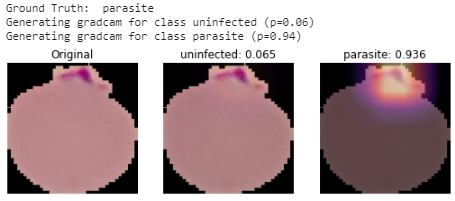
When building a predictive model, there are two important criteria: predictive accuracy and interpretability, which generally have a trade-off relationship. In the previous post, we have shown that the DenseNet121 model can achieve high accuracy in detecting cells infected with parasites.
Here, I am going to introduce a powerful technique GRAD-CAM (gradient-weighted class activation mapping) to visualize which parts of an image are most important to the predictions of an image regression network. GRAD-CAM is a generalization of the CAM technique which determines the importance of each neuron in a network prediction by considering the gradients of the target flowing through the deep network. Unlike CAM which requires a particular kind of CNN architecture to perform global average pooling prior to prediction and forces us to change the base model retrain the network. In contrast, GRAD-CAM is accessing intermediate activations in the deep learning model and computing gradients with respect to the class output. For more details, please see.
Workflow:
- Obtain predicted class/index
- Determine which intermediate layer(s) to use. Lower-level convolution layers capture low level features such as edges, and lines. Higher-level layers usually have more abstract information.
- Calculate the gradients with respect to the outout of the class/index
- Generate a heatmap by weighing the convolution outputs with the computed gradients
- Super-impose the heatmap to the original image
Load base model
We first load the base model and will only train the last 4 layers.
def build_model(input_shape=(224, 224,3),pos_weights,neg_weights):
  # load the base DenseNet121 model
  base_model = DenseNet121(input_shape = input_shape,
                      weights='imagenet',
                      include_top=False)

  # add a GAP layer
  output = layers.GlobalAveragePooling2D()(base_model.output)

  # output has two neurons for the 2 classes (uninfected and parasite)
  output = layers.Dense(2, activation='softmax')(output)

  # set the inputs and outputs of the model
  model = Model(base_model.input, output)

  # freeze the earlier layers
  for layer in base_model.layers[:-4]:
      layer.trainable=False

  # configure the model for training
  model.compile(loss= get_weighted_loss(neg_weights, pos_weights),
                optimizer=adam,
                metrics=['accuracy'])

  return model
We then create a new model that has the original model’s inputs, but two different outputs. The first output contains the activation layers outputs that in this case is the final convolutional layer in the original model. And the second output is the model’s prediction for the image.
def get_CAM(model, processed_image, actual_label, layer_name):
    """
    GradCAM method for visualizing input saliency.

    Args:
        model (Keras.model): model to compute cam for
        image (tensor): input to model, shape (1, H, W, 3)
        cls (int): class to compute cam with respect to
        layer_name (str): relevant layer in model
        H (int): input height
        W (int): input width
    Return:
        heatmap()
    """

    model_grad = Model([model.inputs],
                       [model.get_layer(layer_name).output, model.output])

    with tf.GradientTape() as tape:
        conv_output_values, predictions = model_grad(processed_image)

        # assign gradient tape to monitor the conv_output
        tape.watch(conv_output_values)

        # use binary cross entropy loss, actual_label = 0 if uninfected
        # get prediction probability of infected
        pred_prob = predictions[:,1]

        # make sure actual_label is a float, like the rest of the loss calculation
        actual_label = tf.cast(actual_label, dtype=tf.float32)

        # add a tiny value to avoid log of 0
        smoothing = 0.00001

        # Calculate loss as binary cross entropy
        loss = -1 * (actual_label * tf.math.log(pred_prob + smoothing) + (1 - actual_label) * tf.math.log(1 - pred_prob + smoothing))
        print(f"binary loss: {loss}")

    # get the gradient of the loss with respect to the outputs of the last conv layer
    grads_values = tape.gradient(loss, conv_output_values)
    grads_values = K.mean(grads_values, axis=(0,1,2))

    conv_output_values = np.squeeze(conv_output_values.numpy())
    grads_values = grads_values.numpy()

    # weight the convolution outputs with the computed gradients
    for i in range(grads_values.shape[-1]):
        conv_output_values[:,:,i] *= grads_values[i]
    heatmap = np.mean(conv_output_values, axis=-1)

    heatmap = np.maximum(heatmap, 0)
    heatmap /= heatmap.max()

    del model_grad, conv_output_values, grads_values, loss

    return heatmap
Note:
Instead of using max pooling that only keeps the highest valued ones. Average pooling allows some of the lesser intensity pixels to pass on in the pooling layer. It is important as we look at the small size of the image once it reaches this layer, max pooling could leave us with very little information.

Leave a comment