I remember years ago seeing my colleague spent hours under a microscopes counting cells underwent of apoptosis or Dauer larva formation. I mean it is fun doing experiments in the lab but telling differences of these tiny worms would probably is the last thing I’d want to do. This task does take lots of valuable time from a researcher. Imagine, how many more novel anti-agents like this article Yongsoon could bring us if the deep learning techniques were ready to use back in 2011.
Thanks to the advancement in deep learning field, neural network model architectures can be readily reused and, in most cases, are tested across multiple applications to establish robustness. Here, I’m going to show how easy it is to implement transfer learning using Keras in Python for Malaria cell classification. The basic concept of transfer learning is using the knowledge (architecture or weights) gained from a neural network model that was trained to recognize animals to recognize cats. The dataset used here came from NIH, along with recent publications1,2.
Workflow
- Loading data and data pre-processing
- Transfer learning and fine-tuning (DenseNet121)
- Result evaluation
Data Overview
There are many ways to create train/valid/test data sets. Below is one of the methods using R to create csv files containing file paths and classifications from train and test folders.
# R code
library(fs)
dataset_dir <- "Data/cell_images/"
test_dir   <- paste0(dataset_dir, "/test/")
# stored image paths in the image column
test_parasite <- dir_ls(path=paste0(test_dir, "parasite"),glob = "*.png")
test_uninfected <- dir_ls(path=paste0(test_dir, "uninfected"),glob = "*.png")
test_par <- as.data.frame(matrix('parasite', length(test_parasite), 1))
test_unin <- as.data.frame(matrix('uninfected', length(test_parasite), 1))
test_par$image <- test_parasite
test_unin$image <- test_uninfected

test <- rbind(test_par,test_unin)
colnames(test)[1] <- 'label'
test$normal  <- ifelse(test$label != 'parasite', 1,0)
test$parasite <- ifelse(test$label == 'parasite', 1,0)
And the csv file looks like this.
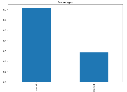
In reality, we don’t usually see many cells infected with parasites, therefore less than 1/3 of the infected samples were used in this exercise.
# Python
# get ids for each label
all_img_ids = list(new_df.uninfected.index.unique())
train_ids, test_ids = train_test_split(all_img_ids, test_size=0.01, random_state=21)
train_ids, valid_ids = train_test_split(train_ids, test_size=0.1, random_state=21)
Making sure, the proportion of the infected cell is as expected after data split.
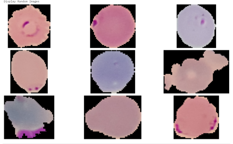
Let’s also check few images. The images come with different sizes. They will need to reshape and normalize before xx.
# Extract numpy values from image column in data frame
train_df = new_df.iloc[train_ids,:]
images = train_df['image'].values
# Extract 9 random images
random_images = [np.random.choice(images) for i in range(9)]
img_dir = 'C:/Users/your_image_folder'
print('Display Random Images')
# Adjust the size of your images
plt.figure(figsize=(20,10))
for i in range(9):
    plt.subplot(3, 3, i + 1)
    img = plt.imread(os.path.join(img_dir, random_images[i]))
    plt.imshow(img)
    plt.axis('off')
Loading data
Next is building generators from the Keras framework. The purpose of building generator is that it allows to generate batches of tensor image data with real-time data augmentation(ex: random horizontal flipping of images). We also use the generator to transform the values in each batch so that their mean is 0 and their standard deviation is 1.Here is the information of ImageDataGenerator and a short tutorial. We’ll also need to build a sereperate generator for valid and test sets. Since each image will be normailized using mean and standard deviation derived from its own batch. In a real life scenario, we process one image at a time. And the incoming image is normalized using the statistics computed from the training set.
# Train generator
def get_train_generator(df, image_dir, x_col, y_cols, shuffle=True, batch_size=8, seed=1, target_w = 224, target_h = 224):
    """

    Args:
      train_df (dataframe): dataframe specifying training data.
      image_dir (str): directory where image files are held.
      x_col (str): name of column in df that holds filenames.
      y_cols (list): list of strings that hold y labels for images.
      sample_size (int): size of sample to use for normalization statistics.
      batch_size (int): images per batch to be fed into model during training.
      seed (int): random seed.
      target_w (int): final width of input images.
      target_h (int): final height of input images.

    Returns:
        train_generator (DataFrameIterator): iterator over training set
    """
    print("getting train generator...")
    # normalize images
    image_generator = ImageDataGenerator(
        samplewise_center=True,
        samplewise_std_normalization= True)

    # flow from directory with specified batch size and target image size
    generator = image_generator.flow_from_dataframe(
            dataframe=df,
            directory=image_dir,
            x_col=x_col,
            y_col=y_cols,
            class_mode="raw",
            batch_size=batch_size,
            shuffle=shuffle,
            seed=seed,
            target_size=(target_w,target_h))

    return generator
Before, model building we’ll need to define a loss function to adress class imbalance. We can give more weight for the less frequent class and less weight for the other one, see here . We can write the overall average cross-entropy loss over the entire training set D of size N as follows:
Next, we will use a pre-trained DenseNet121 model which we can load directly from Keras and then add two layers on top of it.
-
Set include_top=False, to remove the orginal fully connect dense layer (so you can adjust the ouptut prediction clsses or
activation function). -
Use specific layer using get_layer(). For example: base_model.get_layer(‘conv5_block16_conv’)
A GlobalAveragePooling2D layer to get the average of the last convolution layers from DenseNet121. The pooling layer typically uses a filter to extract representative features (e.g., maximum, average, etc.) for different locations. The method of extracting features from the pooling filter is called a pooling function. The commonly used pooling functions include the maximum pooling function, average pooling function, L2 normalization, and weighted average pooling function based on the distance from the center pixel. In short, the pooling layer summarizes all the feature information centered on each position of the input feature map, which makes it reasonable that the output data of the pooling layer is less than the input data. This method reduces the input data to the next layer and improves the computational efficiency of the CNN.
The output of the pooling layer is flattening to convert the pooled features maps into a single dimensional array. This is done in order for the data to be fed into densely connected hidden layers.
A Dense layer with sigmoid activation to get the prediction logits for each of our classes. We can set our custom loss function for the model by specifying the loss parameter in the compile() function.
# Build model
def create_dense121_model():

    pretrained = 'fine_tuned.hdf5'
    train_df = pd.read_csv("train_df.csv")
    labels = ['uninfected', 'parasite']

    class_pos = train_df.loc[:, labels].sum(axis=0)
    class_neg = len(train_df) - class_pos
    class_total = class_pos + class_neg

    pos_weights =  class_pos / class_total #[0.5,class_pos / class_total]
    neg_weights =  class_neg / class_total #[0.5,class_neg / class_total]
    print("Got loss weights")

    def create_model(input_shape=(224, 224,3)):
        base_model = DenseNet121(weights='imagenet', include_top=False, input_shape=input_shape)

        # add a global spatial average pooling layer
        x = GlobalAveragePooling2D()(base_model.output)
        x = Flatten()(x)
        x = Dense(1024, activation='relu', name='dense_post_pool')(x)
        x = Dropout(0.8)(x)
        # output has two neurons for the 2 classes (uninfected and parasite)
        predictions = Dense(len(labels), activation='sigmoid')(x)
        model = Model(inputs = base_model.input, outputs = predictions)

        # freeze the earlier layers
        for layer in base_model.layers[:-4]:
            layer.trainable=False

        return model

    def get_weighted_loss(neg_weights, pos_weights, epsilon=1e-7):
        def weighted_loss(y_true, y_pred):
            y_true = tf.cast(y_true, tf.float32)
            #print(f'neg_weights : {neg_weights}, pos_weights: {pos_weights}')
            #print(f'y_true : {y_true}, y_pred: {y_pred}')
            # L(X, y) = −w * y log p(Y = 1|X) − w *  (1 − y) log p(Y = 0|X)
            # from https://arxiv.org/pdf/1711.05225.pdf
            loss = 0

            for i in range(len(neg_weights)):
                loss -= (neg_weights[i] * y_true[:, i] * K.log(y_pred[:, i] + epsilon) +
                         pos_weights[i] * (1 - y_true[:, i]) * K.log(1 - y_pred[:, i] + epsilon))

            loss = K.sum(loss)
            return loss
        return weighted_loss


    model = create_model()
    model.load_weights(pretrained)
    print("Loaded Model")

    model.compile(optimizer='adam', loss= get_weighted_loss(neg_weights, pos_weights))
    print("Compiled Model")

    return model
Model is fine tuned using ModelCheckpoint and only the model’s weights will be saved.
# CallBack
# -------------------------------------------------------------------------------------------------
# Callback Function 1
fname = 'dense121(V)_Epoch[{epoch:02d}].ValLoss[{val_loss:.3f}].hdf5'
fullpath = fname
# https://keras.io/api/callbacks/model_checkpoint/
callback_func1 = ModelCheckpoint(filepath=fullpath,
                                monitor='val_loss',
                                verbose=1,
                                save_best_only=True,
                                save_weights_only=True, # save weights
                                mode='min',
                                period=1)

# Callback Function 2
# https://keras.io/callbacks/#tensorboard
callback_func2 = keras.callbacks.TensorBoard(log_dir='./logs/log2', histogram_freq=1)

# Callback Function
callbacks = []
callbacks.append(callback_func1)
callbacks.append(callback_func2)

# Training and Plotting
# -------------------------------------------------------------------------------------------------
history = model.fit(train_generator,
                              validation_data=valid_generator,
                              steps_per_epoch=100,
                              validation_steps=25,
                              epochs = 15,
                              callbacks=callbacks)

plt.plot(history.history['loss'])
plt.plot(history.history['val_loss'])
plt.ylabel("loss")
plt.xlabel("epoch")
plt.title("Training Loss Curve")
plt.show()
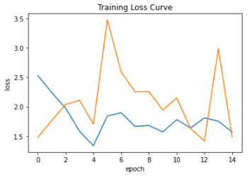
Train versus validation loss for all epochs is shown here. The orange and blue lines indicate train loss and validation loss respectively. We can see the model may be under-fitted. One way to overcome this is simply increase the number of epochs. Also with the callback function, we can re-use the best weights saved at 12th epoch.
Evaluation
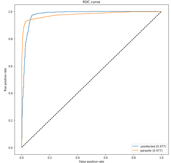
The ROC curve is created by plotting the true positive rate against the false positive rate. We can see the model performs reasonable well.
We can try different approaches to improve the model perfromance, such as train the model for a longer time or use all the training data (since only 1/3 of the parasite data was used). We can also try a different base model, the previous publication, shows 99.32% accuracy with VGG-19 alone.
Visualize class activation maps
Next, I will show how to produce visual explanation using Grad-CAM. The purpose of doing this is as following:
- Debug your model and visually validate that it is “looking” and “activating” at the correct locations in an image.
- Grad-CAM works by (1) finding the final convolutional layer in the network and then (2) examining the gradient information flowing into that layer.
Notes
Note 1: AUC is the area below these ROC curves. Therefore, in other words, AUC is a great indicator of how well a classifier functions. Note 2: A good tutorial for to learn neural network image classification from scratch and Andrew Ng’s deep learning course.
Note 3:
# packages used
import os
import sklearn
import pandas as pd
import numpy as np
import seaborn as sns
import matplotlib.pyplot as plt

import keras
from keras.applications.densenet import DenseNet121
from keras.models import Model
from keras.layers import Dense, Activation, Flatten, Dropout, BatchNormalization, GlobalAveragePooling2D
from keras.callbacks import ModelCheckpoint, CSVLogger, LearningRateScheduler, ReduceLROnPlateau, EarlyStopping, TensorBoard
from keras import backend as K
from keras.preprocessing import image
from keras.preprocessing.image import ImageDataGenerator




Leave a comment